

The list of past posts including those previously published on Wordpress is available here.
Back in November 2025, when doing tests of C4 on a loopback address, I observed that C4 achieved lower data rates than Cubic or even BBR. Since “performance under loopback” was not a high priority scenario, I filed that in the long pile of issues to deal with later. Then, in early January 2026, I read a preprint of a paper by Kathrin Elmenhorst and Nils Aschenbruck titled “2BRobust – Overcoming TCP BBR Performance Degradation in Virtual Machines under CPU Contention” (see: https://arxiv.org/abs/2601.05665). In that paper, they point out that BBR achieves lower than nominal performance when running on VMs under high CPU load, and trace that to pacing issues. Pacing in an application process involves periodically waiting until the pacing system acquires enough tokens. If the CPU is highly loaded, the system call can take longer than the specified maximum wait time, and pacing thus slows the connection more than expected. In such conditions, they suggest increasing the programmed pacing rate above the nominal rate, and show that it helps performance.
C4 is different from BBR, but like BBR it relies on pacing. After reading the paper, I wondered whether similar fixes might be working for C4 as well, and I quickly set up a series of tests.
As mentioned, the first performance tests on C4 over the loopback interface showed lower performance than both BBR and C4. I repeated the tests after modifying the test program to capture a log of the connection in memory, so as to interfere as little as possible with performance.
The memory log showed that the connection was almost always saturating the allocated CWND. That’s not the expected behavior with C4. The CWND is computed as the product of the “nominal rate” and the “nominal max RTT”, which is supposedly higher than the average RTT. When that works correctly, traces show the bytes in flight constantly lower than the program CWND. The CWND is mostly used as some kind of “safety belt”, to limit excess sending in abnormal network conditions.
Looking at the details of the logs showed that the pacing rate was set at a reasonable value, but that the “nominal max RTT” was closely tracking the RTT variations, which oscillated between a few microseconds and up to 1ms. C4 has an adaptive algorithm to draw down the nominal max RTT over time, and after a few RTT that value was getting small, resulting in small values of CWND and low performance.
Our first fix was to set a 1ms floor on max RTT. This will limit the effect of measurement errors and ensure that the CWND always enable 1ms of continuous transmission. We can do this fix safely because C4 enforces pacing at or near the nominal rate, and thus avoids excessive queues that could lead to packet losses.
The effect was immediate. Before the fix, the throughput values observed during loopback tests were both very low and variable. After the fix of the max RTT, the observed throughputs became systematically better than what we observe with BBR on the same computer, and within 88% of the values achieved with Cubic.
Bringing the performance of C4 on loopback within 88% of the performance of Cubic was a great improvement, but why not improve further and reach parity or better?
Kathrin Elmenhorst and Nils Aschenbruck observed that the poor performance of BBR is some scenarios was due to excessive pacing. C4 uses a pacing logic very similar to BBR, and we see that both C4 and BBR performed less well than Cubic in loopback tests. Using memory logs, we verified that the rate estimates were generally lower than the pacing rate, while the theory assumed that they would be almost the same. This is a strong indication that excessive wait time in system calls makes pacing too slow when the CPU is overloaded.
We considered measuring these waiting times, and then developing an automated way to increase the pacing rate above the nominal rate when the waiting times are excessive. The problem is that such adaptive systems are difficult to properly tests, and the time allocated to completing this study was limited. Instead, we use a simple series of tests to check what happens if we increase the pacing rate.
We tested pacing at a fraction above the nominal rate, and we tried three fractions: 1/32, 1/16, and 3/64. Each test showed an improvement. The smaller fraction, 1/32, was bringing the performance close to those of Cubic. The larger fraction, 1/16, was improving on that but was probably excessive: we observed a large amount of packet losses, due to the building of queues. The middle ground actually improved over both previous tests. The observed throughput was better than both the 1/32 and the 1/16 test: higher throughput, but not so high that it would cause excessive losses that slow the transmission. In fact, the performance were now better with C4 than with Cubic.
The graph above shows the resulting performance measured on loopback on a Windows laptop. We did three tests for each congestion control variant, each time measuring the time needed to transfer 10GB and computing the resulting throughput. In the first series of tests, before improvements, C4’s performance was very bad. After setting a floor to the max RTT, performance became better than BBR, but still lower than Cubic. After adding a 3/64th increase to the pacing rate, performance became better than Cubic.
The C4 code in picoquic was fixed to always apply the 1ms floor to the RTT, but to only apply the 3/64th increase if the average RTT is less than 1ms. This restriction ensure that the increase is only used in the narrow conditions under which it was tested, without impeding other scenarios. We could replace that by a more general solution in the future, once we have validated an automated algorithm to detect and compensate for excessive pacing.
Our new congestion control algorithm, C4, is designed to work well in difficult network conditions, and in particular on Wi-Fi networks exhibiting high delay jitter. We noticed the “Wi-Fi jitter” issue two years ago (see the weird case of Wi-Fi latency spikes). We would see sudden jumps in measured RTT, from 1 or 2 milliseconds to 50 tor even 200ms. Since that, we have been looking for explanations of these observation. Our early hypotheses were that the whole Wi-Fi operation was “suspended” for short intervals, either to allow the Wi-Fi device to explore alternative radio frequencies, or perhaps to comply with regulations requiring that Wi-Fi yields to higher priority radio applications like radars at airports. Analyzing more recent traces allowed us to make progress, and explain the phenomenon without the “suspension” hypothesis.

The graph above shows the evolution of RTT over a 75 second connection. It was captured using an ad hoc tool, octoping, that sent udp packets from a client to a responder and recorded the time at which an echo of these packets arrived. The session starts at a point where the transmission conditions are relatively good, before the device moves to a location where Wi-Fi conditions are very degraded and cause numerous delay spikes.

The histogram shows that most measured RTT are small, but that the distribution of RTT has a very long tail, and some kind of exponential distribution.

Looking further, we plotted the observed RTT as a function of the next RTT. That graph has a very distinctive shape, and a very interesting feature, with lots of high value samples clustered around a parallel to the diagonal that crosses the x-axis near the 20 millisecond mark. The rightmost points on that line are spaced 20ms apart. We know that the octoping program sent packets at 20ms intervals. What we see here is a consequence of in order delivery. If the first packet encountered a long RTT, the packet after that, sent 20ms after it, arrives at almost the same time, as if it was retained by some Wi-Fi component until it could be delivered in sequence.

Of course, we don’t want to draw conclusions from just one sample. We have collected multiple such samples, and we do see variations between them, such as the difference showing between in cumulative frequency distributions of observed RTT in three different trials. One of this trials was done in good conditions, and it markedly differs from the other two, with the CFD showing most values clustered around the median. The other two are similar, with a much wider distribution of observed RTT, one being somewhat worse than the other.

To try get a better understanding, we took all the samples. We filtered out values that only differed from the previous observation by the interval between two probes, because in those cases the delays result from in sequence delivery rather that a random process. Then we draw the histogram of all observed values… and it does not tell us much. The leftmost part of the histogram looks like some kind of Gaussian or Poisson process, but the tail is a bit large.

The graph that we found most informative takes the same RTT values per interval, and plots then in a log scale. We seem to have a complex process, combining a short term random process of some sort, and a secondary process that produces very large values, albeit at a low frequency.
We don’t really know what caused this, but we can think of two Wi-Fi processes, both figuring exponential backoff. The CDMA process enables multiple stations managed by different access points to share the same channel. In case of collision, they will retry at a random time picked in an interval that doubles after each collision. The CDMA collisions are generally resolved in a few milliseconds. We believe that CDMA collisions explain the left most part of the curve.
The “bumps” in the right side of the curve have to be explained by a different process that also involves exponential backoff and probably operates with a granularity measured in tens of milliseconds. This could well be due to the “frame retransmission” process that Wi-Fi device uses for the “best effort” channel. If the packet is lost, it is resent after an interval. In case of repeated losses, the repeat interval increases exponentially.
This packet repeat process is not present all the time – for example, we do not see it in the “good” trial in our graph of CFD in three different trials. We see it a lot in the “bad” samples. They were captured in a multi-appartment building. It is very likely that multiple Wi-Fi access points were operating inthat building, causing some packet collisions due to the “hidden terminal” problem.

Whatever the actual cause, we do observe some pretty extreme values of RTT jitter in some Wi-Fi networks. Our first observation is that this jitter is not properly modelled by the algorithm in TCP or QUIC. For example, for QUIC, the algorithm defined in RFC 9002 compute a “smoothed RTT” by performing a exponential smoothing of RTT samples, and a “PTO” timer as the sum of the smoothed RTT and four times the estimated “RTT variance”. We programmed these formulas, and computed the PTO timer for the various traces that we collected. This timer will “fire” when the next acknowledgment does not arrive before its expiration. In the graph, we show the effect for our “near far” trial. Each blue “+” sign correspond to one RTT sample. Each red dot correspond to a firing of the PTO timer. That’s a lot of firings!
In practice, the first effect of these spurious PTO timers will be to mislead the “delay based” algorithms such as Hystart, causing an early exit of the “slow start” phase that is hard for algorithms like Cubic to compensate. We first noticed this problem in 2019 when testing Cubic for QUIC (see Implementing Cubic congestion control in Quic). It is interesting that this blog includes a graph of observed delays very similar to the WiFi trials discussed here, although at the time we focused mostly on the short-scale variations. The low-pass filtering recommended in this blog does solve the short-scale issue, but is defeated by the arrival of very large RTT. After our tests, we fixed our implementation of Cubic to return to slow start if the exit of Hystart was causes by a spurious timer, and that markedly improved the robustness of Cubic.
The second effect is to create large gaps in received packets. Supposed that a packet is delivered with a long latency. All packets sent after it will be queued, and example of “head of line” blocking. This will be perceived by the endpoint as a “suspension”, as we diagnosed in 2023. These gaps will have different effects on different congestion control algorithms. These effects need to be studied. We have thus developed an way to simulate these latencies, so that we can perform tests and simulations of algorithms operating in different Wi-Fi conditions.

We are still not quite sure of the processes causing this latency, but this should not prevent us from doing an useful model that more or less mimics the latency variations of Wi-Fi networks. After all, the models used by Hellenistic astronomers to predict the movement of planets where not exactly based on the formulas later refined by Kepler and then Newton, but their complex combinations of epicycloids was precise enough to build devices like the Antikythera mechanism and help ancient mariners navigate.
In our model, we define the latency by combining several generators, combined using a coefficient x defining how of a secondary long scale repetition is also used:
The latency for a single sample will be:
latency = N1*1ms + N2*7.5ms
if N1 >= 1:
    latency -= r
The coefficient x is derived from the target average jitter value. If the target is 1ms or less, we set x to zero. If it is higher than 91ms, we set x to 1. If it is in between, we set:
x = (average_jitter - 1ms)/90ms
We have been using this simulation of jitter to test our implementation of multiple congestion control algorithms, and to guide the design of C4.
For the past 6 months, I have been working on a new congestion control algorithm, called C4 for “Christian’s Congestion Control Code”, together with Suhas Nandakumar and Cullen Jennings at Cisco. Our goal is to design a congestion control algorithm that serves well real time communication applications, and is generally suitable for use with QUIC. This leads to the following priorities:
Out of those three priorities, the support for “questionable” Wi-Fi had a major influence on the design. We got reports of video not working well in some Wi-Fi networks, notably networks in office buildings shared by multiple tenants and appartment buildings. Analyzing traces showed that these networks could exhibit very large delay jitter, as seen in the following graph:
In presence of such jitter, we see transmission sometimes stalling if the congestion window is too small. To avoid that, we have to set the congestion window to be at least as large as the product of the target data rate by the maximum RTT. This leads to our design decision of tracking two main state variables in C4: the “nominal data rate”, which is very similar to the “bottleneck bandwidth” of BBR (see BBR-draft); and the “nominal max RTT” which is set to the largest recently experienced RTT as measured in the absence of congestion.
The support for application limited flows is achieved by keeping the nominal data rate stable in periods of low application traffic, and only reducing it when congestion is actually experienced. C4 keeps the bandwidth stable by adopting a cautious bandwidth probing strategy, so that in most cases probing does not cause applications to send excess data and cause priority inversions.
C4 uses a “sensitivity” curve to obtain fairness between multiple connections. The sensitivity curve computes sensitivity as function of the nominal data rate, ensuring that flows sending at a high data rate are more sensitive than flows using a lower data rate, and thus reduce their data rate faster in response to congestion signals. Our simulations shows that this drives to fair sharing of a bottleneck between C4 flows, and also ensure reasonable sharing when sharing the bottleneck with Cubic or BBR flows.
We have published three IETF drafts to describe the C4 design, C4 algorithm specifications, and the testing of C4. The C4 repository on Github contains our C implementation of the algorithm, designed to work in Picoquic, as well as testing tools and a variety of papers discussing elements of the design.
The code itself is rather simple, less than 1000 lines of C including lots of comments, but we will need more than one blog post to explain the details. Stay tuned, and please don’t hesitate to give us feedback!
This morning, I was contacted by Victor Stewart, who has been contributing to picoquic for a long time. Victor is using the new Codex extension that OpenAI released last week. He was impressed with the results and the amazing gains in productivity.
I started from a very skeptical point of view. I saw initial attempts at using various AI systems to generate code, and they required a rather large amount of prompting to create rather simple code. I have read reports like Death by a thousand slops by Daniel Steinberg, who rails about sloppy bug reports generated by AI. So I asked Victor whether we could do a simple trial, such as fixing a bug.
Victor picked one of the pending bugs in the list of issues, issue #1937. I had analyzed that bug before, but it was not yet fixed. So we tried. While we were chatting over slack, Victor prompted Codex, and got a first reply with an explanation of the bug and a proposed fixed, more or less in real time. I asked whether it could generate a regression test, and sure enough it did just that. Another prompt to solve some formatting issues, and voila, we got a complete PR.
I was impressed. The fix itself is rather simple, but even for simple bugs like that we need to spend time analysing, finding the repro, writing a regression test, and writing a patch. We did all that in a few minutes over a chat. It would probably have required at least a couple hours of busy work. The Codex system requires a monthly subscription fee, and probably spending some time learning the tool and practicing. But when I see this kind of productivity gain, I am very tempted to just buy it!
The Great Firewall Report, a “long-term censorship monitoring platform”, just published an analysis of how the “Great firewall” handles QUIC. I found that a very interesting read.
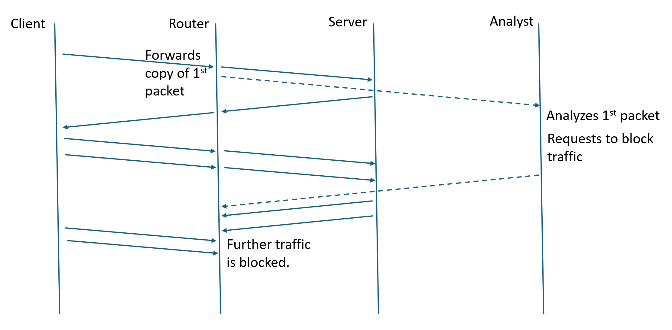
The firewall work is distributed between an analysis center and cooperating routers, presumably at the “internet borders” of the country. The router participation appears simple: monitor incoming UDP flows, as defined by the source and destination IP addresses and ports; capture the first packet of the flow and send it to the analysis center; and, receive and apply commands by the analysis center to block a given flow for 2 minutes. The analysis center performs “deep packet inspection”, looks at the “server name” parameter (SNI), and if that name is on a block list, sends the blocking command to the router.
The paper finds a number of weaknesses in the way the analysis is implemented, and suggests a set of techniques for evading the blockage. For example, clients could send a sacrificial packet full of random noise before sending the first QUIC packet, or they could split the content of the client first fly across several initial packets. These techniques will probably work today, but to me they feel like another of the “cat and mouse” game that gets plaid censors and their opponents. If the censors are willing to dedicate more resource to the problem, they could for example get copies of more than one of the first packets in a stream and perform some smarter analysis.
The client should of course use Encrypted Client Hello (ECH) to hide the name of the server, and thus escape the blockage. The IETF has spent 7 years designing ECH, aiming at exactly the “firewall censorship” scenario. In theory, it is good enough. Many clients have started using “ECH greasing”, sending a fake ECH parameter in the first packet even if they are not in fact hiding the SNI. (Picoquic supports ECH and greasing.) ECH greasing should prevent the firewall from merely “blocking ECH”.
On the other hand, censors will probably try to keep censoring. When the client uses ECH, the “real” SNI is hidden in an encrypted part of the ECH parameter, but there is still an “outer” SNI visible to observers. ECH requires that client fills this “outer” SNI parameter with the value specified by the fronting server in their DNS HTTPS record. We heard reports that some firewalls would just collect these “fronting server SNI values” and add them to their block list. They would block all servers that are fronted by the same server as a one of their blocking targets. Another “cat and mouse” game, probably.